Design linear feedback controller
Let us now create a linear feedback controller that will stabilize the pendulum system that was created in the last section to its upright, unstable equilibrium.
Create pendulum system
Let us start by using the same code from the last section that creates a simple pendulum system with the addition of just a few lines.
# Import necessary python modules
import math
from math import pi
import numpy as np
from numpy import dot
import trep
import trep.discopt
from trep import tx, ty, tz, rx, ry, rz
import pylab

# Build a pendulum system
m = 1.0 # Mass of pendulum
l = 1.0 # Length of pendulum
q0 = 3./4.*pi # Initial configuration of pendulum
t0 = 0.0 # Initial time
tf = 5.0 # Final time
dt = 0.1 # Sampling time
qBar = pi # Desired configuration
Q = np.eye(2) # Cost weights for states
R = np.eye(1) # Cost weights for inputs

system = trep.System() # Initialize system

frames = [
    rx('theta', name="pendulumShoulder"), [
        tz(-l, name="pendulumArm", mass=m)]]
system.import_frames(frames) # Add frames

# Add forces to the system
trep.potentials.Gravity(system, (0, 0, -9.8)) # Add gravity
trep.forces.Damping(system, 1.0) # Add damping
trep.forces.ConfigForce(system, 'theta', 'theta-torque') # Add input

# Create and initialize the variational integrator
mvi = trep.MidpointVI(system)
mvi.initialize_from_configs(t0, np.array([q0]), t0+dt, np.array([q0]))
Three additional (highlighted above) modules are imported: dot from the
numpy module, which we will use for matrix multiplication; pylab (part
of the matplotlib project, which is used for
plotting; and trep’s discrete optimization module, trep.discopt.
In addition, a desired configuration value has been set to the variable
qBar. The desired configuration is \(\pi\), which is the pendulum’s
neutrally-stable, upright configuration. Also, correctly-dimensioned, identity
state and input weighting matrices (Q and R respectively) have been
created for the optimization of the linear feedback controller.
Create discrete system
Trep has a module that provides functionality for solving several linear, time-varying discrete linear-quadratic regulation problems (see this page).
TVec = np.arange(t0, tf+dt, dt) # Initialize discrete time vector
dsys = trep.discopt.DSystem(mvi, TVec) # Initialize discrete system
xBar = dsys.build_state(qBar) # Create desired state configuration
To do this, we use our system definition, and a prescribed time vector to create
a trep.discopt.DSystem. This object is basically a wrapper for
trep.System objects and trep.MidpointVI objects to represent
the general nonlinear discrete systems as first order discrete nonlinear systems
of the form \(X(k+1) = f(X(k), U(k), k)\).
The states \(X\) and inputs \(U\) of a trep.discopt.DSystem
should be noted. The state consists of the variational integrator’s full
configuration, the dynamic momentum, and the kinematic velocity. The full
configuration consist of both dynamic states and kinematic states. The
difference being that the dynamic states are governed by first-order
differential equations and the kinematic states can be set directly with
“kinematic” inputs. This is equivalent to saying you have “perfect” control over
a dynamic configuration i.e. your system is capable of exerting unlimited force
to drive the configuration to follow any arbitrary trajectory. The kinematic
velocity is calculated as a finite difference of the kinematic
configurations. The trep.discopt.DSystem class has a method,
trep.discopt.DSystem.build_state, that will “build” this state vector from
configuration, momentum, and kinematic velocity vectors. “Build” here means
construct a state array of the correct dimension. Anything that is not specified
is set to zero. This is used above to calculated a desired state array from the
desired configuration value.
Using IPython you can display a list of all the properties and methods of the discrete system.
>>> dsys.
dsys.build_input               dsys.fdu                       dsys.save_state_trajectory
dsys.build_state               dsys.fdudu                     dsys.set
dsys.build_trajectory          dsys.fdx                       dsys.split_input
dsys.calc_feedback_controller  dsys.fdxdu                     dsys.split_state
dsys.check_fdu                 dsys.fdxdx                     dsys.split_trajectory
dsys.check_fdudu               dsys.k                         dsys.step
dsys.check_fdx                 dsys.kf                        dsys.system
dsys.check_fdxdu               dsys.linearize_trajectory      dsys.time
dsys.check_fdxdx               dsys.load_state_trajectory     dsys.uk
dsys.convert_trajectory        dsys.nU                        dsys.varint
dsys.dproject                  dsys.nX                        dsys.xk
dsys.f                         dsys.project
Please refer to the DSystem documentation to learn more about this object.
Design linear feedback controller
Let us now design a linear feedback controller to stabilize the pendulum to the desired configuration.
Qd = np.zeros((len(TVec), dsys.system.nQ)) # Initialize desired configuration trajectory
thetaIndex = dsys.system.get_config('theta').index # Find index of theta config variable
for i,t in enumerate(TVec):
    Qd[i, thetaIndex] = qBar # Set desired configuration trajectory
    (Xd, Ud) = dsys.build_trajectory(Qd) # Set desired state and input trajectory

Qk = lambda k: Q # Create lambda function for state cost weights
Rk = lambda k: R # Create lambda function for input cost weights
KVec = dsys.calc_feedback_controller(Xd, Ud, Qk, Rk) # Solve for linear feedback controller gain
KStabilize = KVec[0] # Use only use first value to approximate infinite-horizon optimal controller gain

# Reset discrete system state
dsys.set(np.array([q0, 0.]), np.array([0.]), 0)
The DSystem class has a method
(trep.discopt.DSystem.calc_feedback_controller) for calculating a
stabilizing feedback controller for the system about state and input
trajectories given both state and input weighting functions.
A trajectory of the desired configuration is constructed and then used with the
trep.discopt.DSystem.build_trajectory method to create the desired state
and input trajectories. The weighting functions are created with Python lambda
functions that always output the state and input cost weights that were assigned
to Qk and Rk. The calc_feedback_controller method returns the gain
value \(K\) for each instance in time. To approximate the infinite-horizon
optimal controller only the first value is used.
The discrete system must be reset to the initial state value because during the
optimization the discrete system is integrated and thus set to the final
time. Note, because the discrete system was created from the variational
integrator, which was created from the system; setting the discrete system
states also sets the configuration of variational integrator and the
system. This can be checked by checking the values before and after running the
set method, as shown below.
>>> dsys.xk
array([ 3.14159265,  0.        ])
>>> mvi.q1
array([ 3.14159265])
>>> system.q
array([ 3.14159265])
>>> dsys.set(np.array([q0, 0.]), np.array([0.]), 0)
>>> dsys.xk
array([ 2.35619449,  0.        ])
>>> mvi.q1
array([ 2.35619449])
>>> system.q
array([ 2.34019535])
>>> (mvi.q2 + mvi.q1)/2.0
array([ 2.34019535])
Note that the system.q returns the current configuration of the system.
This is calculated using the midpoint rule and the endpoints of the variational
integrator as seen above.
Simulate the system forward
As was done in the previous section of this tutorial the system is simulated forward with a while loop, which steps it forward one time step at a time.
T = [mvi.t1] # List to hold time values
Q = [mvi.q1] # List to hold configuration values
X = [dsys.xk] # List to hold state values
U = [] # List to hold input values
while mvi.t1 < tf-dt:
    x = dsys.xk # Grab current state
    xTilde = x - xBar # Compare to desired state
    u = -dot(KStabilize, xTilde) # Calculate input
    dsys.step(u) # Step the system forward by one time step
    T.append(mvi.t1) # Update lists
    Q.append(mvi.q1)
    X.append(x)
    U.append(u)
This time the system is stepped forward with the
trep.discopt.DSystem.step method instead of the
trep.MidpointVI.step method. This is done so that the discrete state gets
updated and set as well as the system configurations and momenta. The input is
calcuated with a standard negative feedback of the state error multiplied by the
gain that was found previously. In addition, two more variables are created to
store the state values and the input values throughout the simulation.
Visualize the system in action
The visualization is created in the exact way it was created in the last section. But this time also plotting state and input verse time.
trep.visual.visualize_3d([ trep.visual.VisualItem3D(system, T, Q) ])

# Plot results
ax1 = pylab.subplot(211)
pylab.plot(T, X)
pylab.title("Linear Feedback Controller")
pylab.ylabel("X")
pylab.legend(["qd","p"])
pylab.subplot(212, sharex=ax1)
pylab.plot(T[1:], U)
pylab.xlabel("T")
pylab.ylabel("U")
pylab.legend(["u"])
pylab.show()
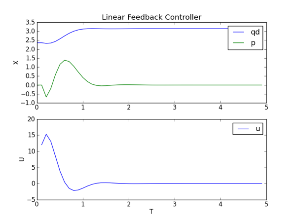
From the plot you can see that it requires a large input to stablize the pendulum. What if the input torque is limited to a smaller value and we want to bring the pendulum to the upright configuration from any other configuration? By using a swing-up controller and then switching to this linear feedback controller we can accomplish this stabilization with a limited input from any configuration. We will demonstrate how this can be done with trep in the next two sections.
linearFeedbackController.py code
Below is the entire script used in this section of the tutorial.
1 2 3 4 5 6 7 8 9 10 11 12 13 14 15 16 17 18 19 20 21 22 23 24 25 26 27 28 29 30 31 32 33 34 35 36 37 38 39 40 41 42 43 44 45 46 47 48 49 50 51 52 53 54 55 56 57 58 59 60 61 62 63 64 65 66 67 68 69 70 71 72 73 74 75 76 77 78 79 80 81 82 83 84 85 86 87 88 89 | # linearFeedbackController.py
# Import necessary python modules
import math
from math import pi
import numpy as np
from numpy import dot
import trep
import trep.discopt
from trep import tx, ty, tz, rx, ry, rz
import pylab
# Build a pendulum system
m = 1.0 # Mass of pendulum
l = 1.0 # Length of pendulum
q0 = 3./4.*pi # Initial configuration of pendulum
t0 = 0.0 # Initial time
tf = 5.0 # Final time
dt = 0.1 # Sampling time
qBar = pi # Desired configuration
Q = np.eye(2) # Cost weights for states
R = np.eye(1) # Cost weights for inputs
system = trep.System() # Initialize system
frames = [
rx('theta', name="pendulumShoulder"), [
tz(-l, name="pendulumArm", mass=m)]]
system.import_frames(frames) # Add frames
# Add forces to the system
trep.potentials.Gravity(system, (0, 0, -9.8)) # Add gravity
trep.forces.Damping(system, 1.0) # Add damping
trep.forces.ConfigForce(system, 'theta', 'theta-torque') # Add input
# Create and initialize the variational integrator
mvi = trep.MidpointVI(system)
mvi.initialize_from_configs(t0, np.array([q0]), t0+dt, np.array([q0]))
# Create discrete system
TVec = np.arange(t0, tf+dt, dt) # Initialize discrete time vector
dsys = trep.discopt.DSystem(mvi, TVec) # Initialize discrete system
xBar = dsys.build_state(qBar) # Create desired state configuration
# Design linear feedback controller
Qd = np.zeros((len(TVec), dsys.system.nQ)) # Initialize desired configuration trajectory
thetaIndex = dsys.system.get_config('theta').index # Find index of theta config variable
for i,t in enumerate(TVec):
Qd[i, thetaIndex] = qBar # Set desired configuration trajectory
(Xd, Ud) = dsys.build_trajectory(Qd) # Set desired state and input trajectory
Qk = lambda k: Q # Create lambda function for state cost weights
Rk = lambda k: R # Create lambda function for input cost weights
KVec = dsys.calc_feedback_controller(Xd, Ud, Qk, Rk) # Solve for linear feedback controller gain
KStabilize = KVec[0] # Use only use first value to approximate infinite-horizon optimal controller gain
# Reset discrete system state
dsys.set(np.array([q0, 0.]), np.array([0.]), 0)
# Simulate the system forward
T = [mvi.t1] # List to hold time values
Q = [mvi.q1] # List to hold configuration values
X = [dsys.xk] # List to hold state values
U = [] # List to hold input values
while mvi.t1 < tf-dt:
x = dsys.xk # Grab current state
xTilde = x - xBar # Compare to desired state
u = -dot(KStabilize, xTilde) # Calculate input
dsys.step(u) # Step the system forward by one time step
T.append(mvi.t1) # Update lists
Q.append(mvi.q1)
X.append(x)
U.append(u)
# Visualize the system in action
trep.visual.visualize_3d([ trep.visual.VisualItem3D(system, T, Q) ])
# Plot results
ax1 = pylab.subplot(211)
pylab.plot(T, X)
pylab.title("Linear Feedback Controller")
pylab.ylabel("X")
pylab.legend(["qd","p"])
pylab.subplot(212, sharex=ax1)
pylab.plot(T[1:], U)
pylab.xlabel("T")
pylab.ylabel("U")
pylab.legend(["u"])
pylab.show()
|